Installation
You can install the stable version of BKP from CRAN with:
install.packages("BKP")Or install the development version from GitHub with:
# install.packages("pak")
pak::pak("Jiangyan-Zhao/BKP")
BKP model
Example 1
Let , and suppose the true Bernoulli probability function is given by
# Define true success probability function
true_pi_fun <- function(x) {
  1/(1+exp(-3*x))
}
X <- seq(-2, 2, length = 1000)
true_pi <- true_pi_fun(X)
plot(X, true_pi, type = "l", lwd = 2, xlab = "x", ylab = "Probability")
We aim to fit the BKP model based on seven input locations that are uniformly distributed over , with each location associated with a binomial observation having a maximum trial count of 100.
set.seed(123)
# Data generation
n <- 7
Xbounds <- matrix(c(-2,2), nrow = 1)
X <- lhs(n = n, rect = Xbounds)
true_pi <- true_pi_fun(X)
m <- sample(100, n, replace = TRUE)
y <- rbinom(n, size = m, prob = true_pi)

# Fit BKP model
BKP_model_1D_1 <- fit.BKP(X, y, m, Xbounds = Xbounds)

# Plot results
plot(BKP_model_1D_1)

# Add true probability function
Xnew = matrix(seq(-2, 2, length = 100), ncol=1)
true_pi <- true_pi_fun(Xnew)
lines(Xnew,true_pi, col = "black", lwd = 2)
legend(x = -2.24,y = 0.89, lwd = 2, bty = "n", col = "black",
       legend = "Ture Probability", inset = 0.02)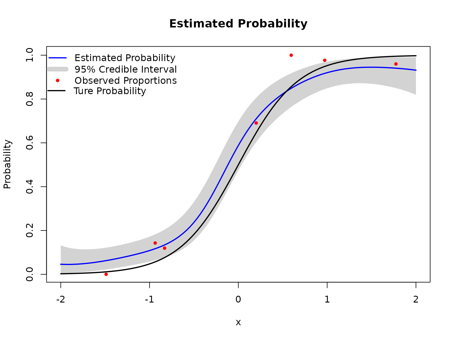
Example 2
The first example is essentially a generalized linear model with a smooth logit link, and thus poses limited modeling complexity. To demonstrate the capability of the BKP model in handling more challenging classification structures, we consider a second example with a highly nonlinear underlying probability surface. Define the true Bernoulli probability as where . This example involves rapid local oscillations and strong nonlinearity, making it substantially more difficult to fit than Example 1. Here, we increase the number of locations to 30.
# Define true success probability function
true_pi_fun <- function(x) {
  (1 + exp(-x^2) * cos(10 * (1 - exp(-x)) / (1 + exp(-x)))) / 2
}
X <- seq(-2, 2, length = 1000)
true_pi <- true_pi_fun(X)
plot(X, true_pi, type = "l", lwd = 2,
     xlab = "x", ylab = "Probability")
set.seed(123)
# Data generation
n <- 30
Xbounds <- matrix(c(-2,2), nrow = 1)
X <- lhs(n = n, rect = Xbounds)
true_pi <- true_pi_fun(X)
m <- sample(100, n, replace = TRUE)
y <- rbinom(n, size = m, prob = true_pi)

# Fit BKP model
BKP_model_1D_2 <- fit.BKP(X, y, m, Xbounds = Xbounds)

# Plot results
plot(BKP_model_1D_2)

# Add true probability function
Xnew = matrix(seq(-2, 2, length = 100), ncol=1)
true_pi <- true_pi_fun(Xnew)
lines(Xnew,true_pi, col = "black", lwd = 2)
legend(x = -2.24,y = 0.89, lwd = 2, bty = "n", col = "black",
       legend = "Ture Probability", inset = 0.02)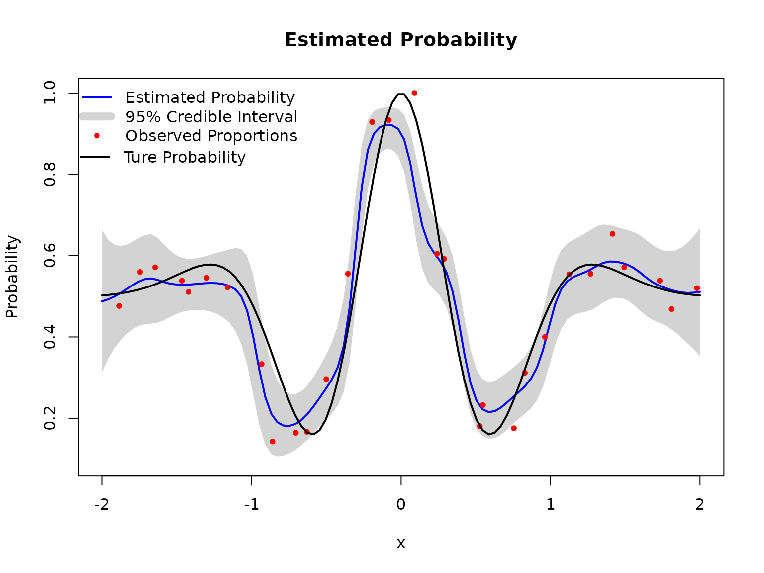
Example 3
Let , and define the latent surface using a re-scaled version of the Goldstein–Price function:
The true Bernoulli probability surface is then defined by where is the cumulative distribution function of the standard normal distribution.
# Define 2D latent function and probability transformation
true_pi_fun <- function(X) {
  if(is.null(nrow(X))) X <- matrix(X, nrow=1)
  m <- 8.6928
  s <- 2.4269
  x1 <- 4*X[,1]- 2
  x2 <- 4*X[,2]- 2
  a <- 1 + (x1 + x2 + 1)^2 *
    (19- 14*x1 + 3*x1^2- 14*x2 + 6*x1*x2 + 3*x2^2)
  b <- 30 + (2*x1- 3*x2)^2 *
    (18- 32*x1 + 12*x1^2 + 48*x2- 36*x1*x2 + 27*x2^2)
  f <- log(a*b)
  f <- (f- m)/s
  return(pnorm(f))  # Transform to probability
}
x1 <- seq(0, 1, length.out = 100)
x2 <- seq(0, 1, length.out = 100)
X <- expand.grid(x1 = x1, x2 = x2)
true_pi <- true_pi_fun(X)
df <- data.frame(x1 = X$x1, x2 = X$x2, True = true_pi)
print(BKP:::my_2D_plot_fun("True", title = "True Probability", data = df))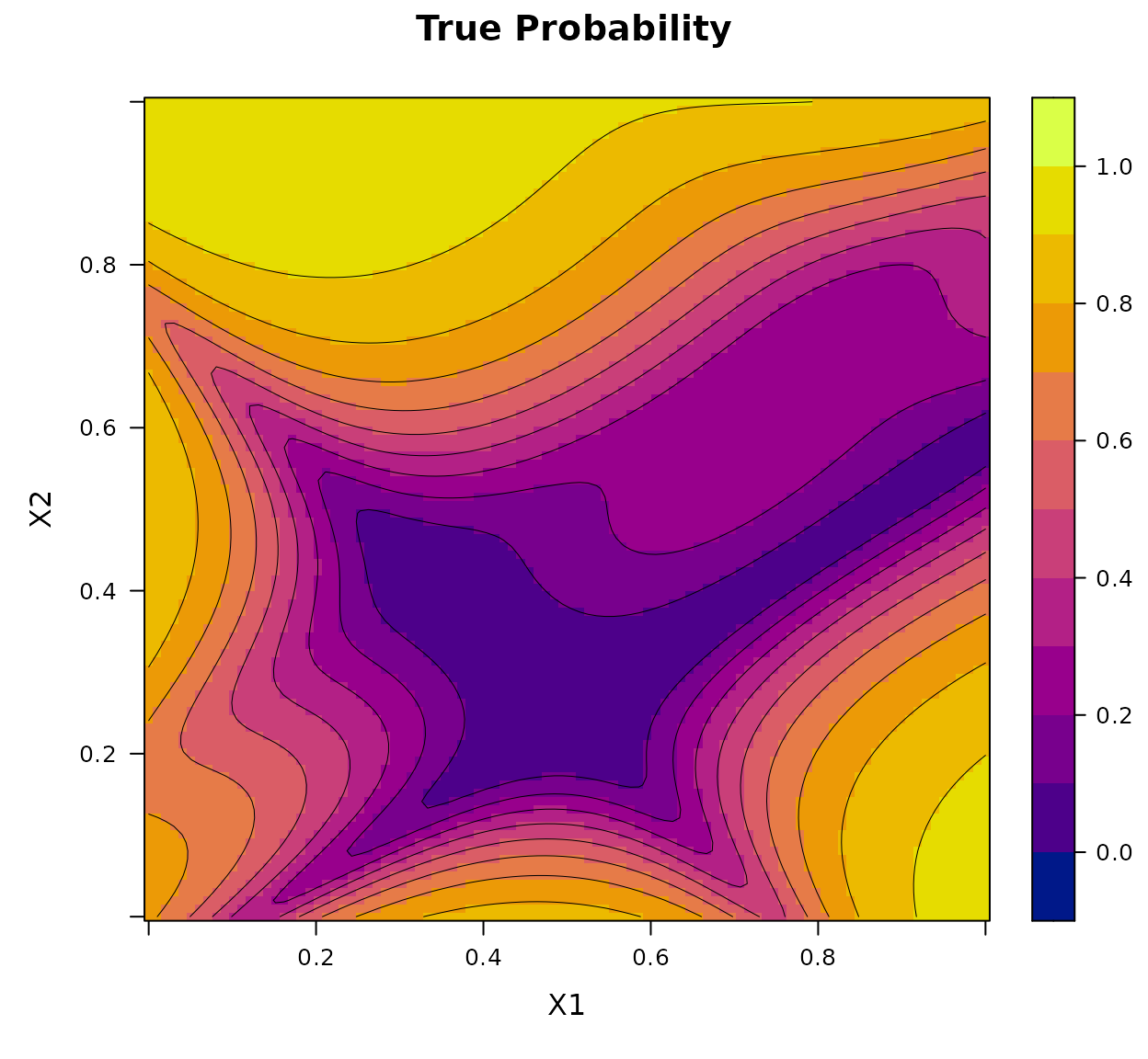
To construct the training data, we generate a LHD of size over . Each location is associated with a binomial observation whose number of trials is randomly drawn from .
set.seed(123)
# Data generation
n <- 100
Xbounds <- matrix(c(0, 0, 1, 1), nrow = 2)
X <- lhs(n = n, rect = Xbounds)
true_pi <- true_pi_fun(X)
m <- sample(100, n, replace = TRUE)
y <- rbinom(n, size = m, prob = true_pi)

# Fit BKP model
BKP_model_2D <- fit.BKP(X, y, m, Xbounds=Xbounds)

# Plot results
plot(BKP_model_2D)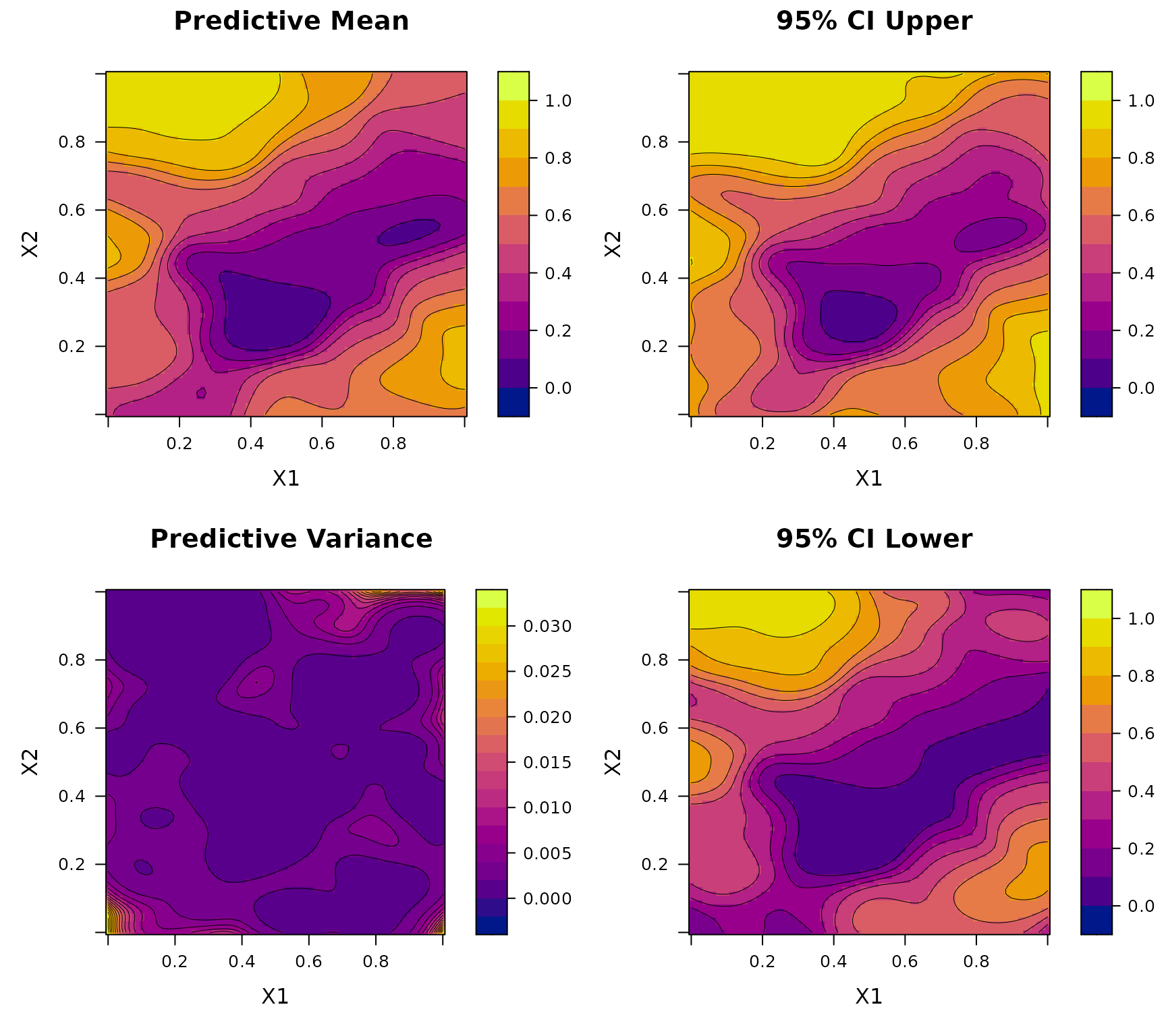
Example 4
We next consider a binary classification task using the Two Spirals dataset, a well-known benchmark consisting of two intertwined spirals in a bounded two-dimensional input space.
We generate
observations using the mlbench.spirals function from the R
package mlbench, with two
complete rotations and additive Gaussian noise of standard deviation
sd = 0.05. The inputs
are constrained to the domain
,
and the binary class labels are encoded as 0 and 1. We fit the BKP model
using a fixed prior specification with r_0 = 0.1 and
p_0 = 0.5.
library(mlbench)
set.seed(123)
# Data
n <- 200
data <- mlbench.spirals(n, cycles = 2, sd = 0.05)
X <- data$x
y <- as.numeric(data$classes) - 1  # Convert to 0/1 for BKP
m <- rep(1, n)
Xbounds <- rbind(c(-1.7, 1.7), c(-1.7, 1.7))

# Fit model
BKP_model_Class <- fit.BKP(
  X, y, m, Xbounds = Xbounds,
  prior = "fixed", r0 = 0.1, loss = "log_loss")

# Plot results
plot(BKP_model_Class)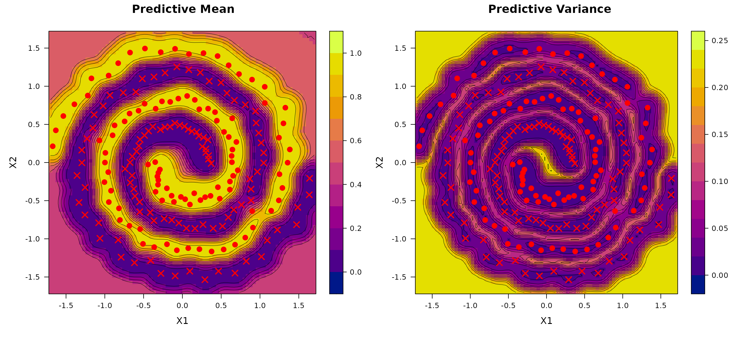
DKP model
Example 5
Consider a one-dimensional three-class classification problem. The input is defined on the interval , and the true class probability vector is given by where and are smooth functions defined in Example 1 and 2, respectively. We generate input locations using Latin hypercube sampling over the interval . At each location, the response is a multinomial vector with probability and a random total count sampled from .
set.seed(123)
# Define true class probability function (3-class)
true_pi_fun <- function(X) {
  p1 <- 1/(1+exp(-3*X))
  p2 <- (1 + exp(-X^2) * cos(10 * (1 - exp(-X)) / (1 + exp(-X)))) / 2
  return(matrix(c(p1/2, p2/2, 1 - (p1+p2)/2), nrow = length(p1)))
}
# Data points
n <- 30
Xbounds <- matrix(c(-2, 2), nrow = 1)
X <- lhs(n = n, rect = Xbounds)
true_pi <- true_pi_fun(X)
m <- sample(150, n, replace = TRUE)
Y <- t(sapply(1:n, function(i) rmultinom(1, size = m[i], prob = true_pi[i, ])))

# Fit DKP model
DKP_model_1D <- fit.DKP(X, Y, Xbounds = Xbounds)

# Plot results
plot(DKP_model_1D)

# Add true probability surface
Xnew <- matrix(seq(-2,2, length = 100), ncol=1)
true_pi <- true_pi_fun(Xnew)
plot(Xnew, true_pi[, 1], type = "l", col = "black",
     xlab = "x", ylab = "Probability", ylim = c(0, 1),
     main = "True Probability", lwd = 2)
lines(Xnew, true_pi[, 2], col = "red", lwd = 2)
lines(Xnew, true_pi[, 3], col = "blue", lwd = 2)
legend("topright",
       bty = "n",
       legend = c("Class 1", "Class 2", "Class 3"),
       col = c("black", "red", "blue"), lty = 1, lwd = 2)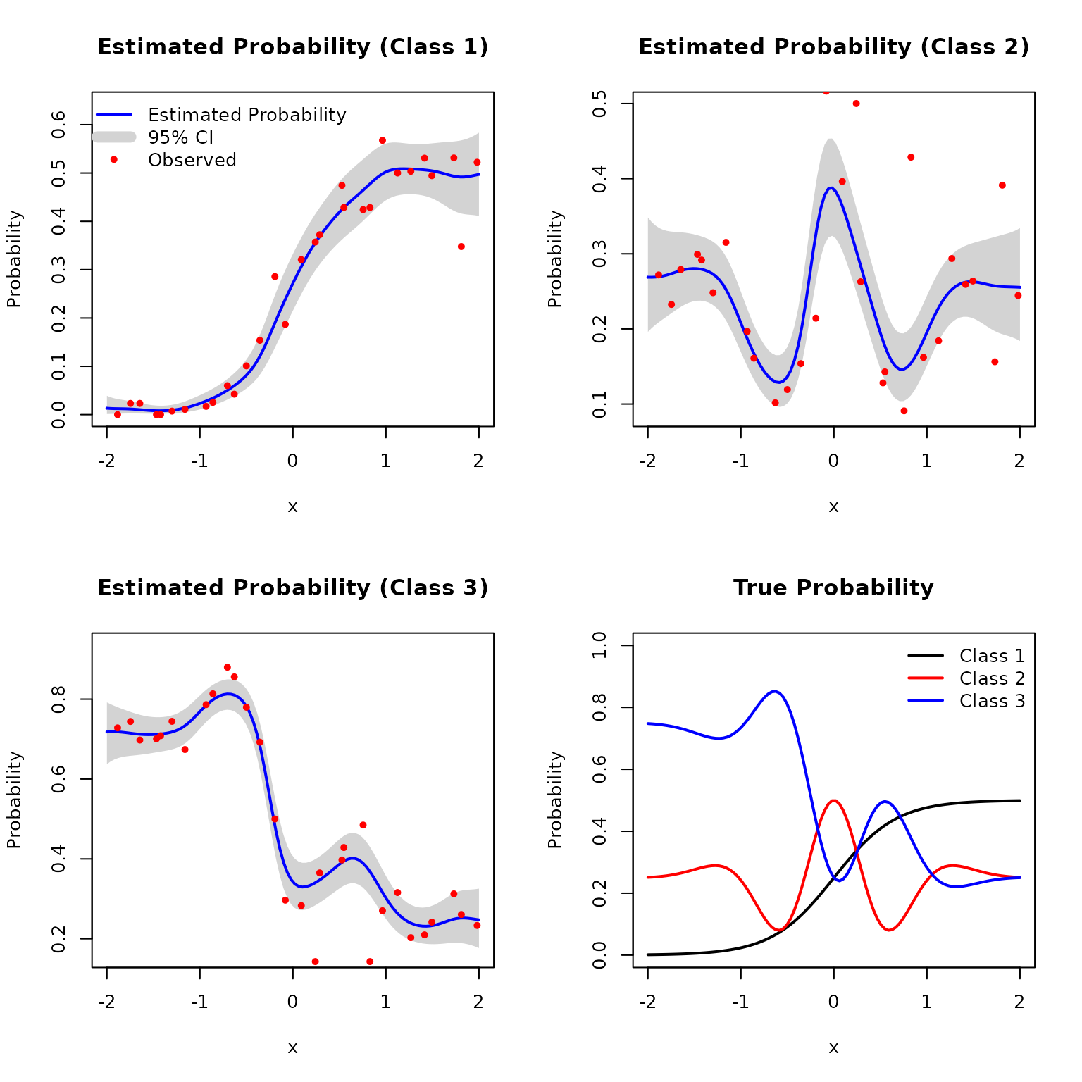
Example 6
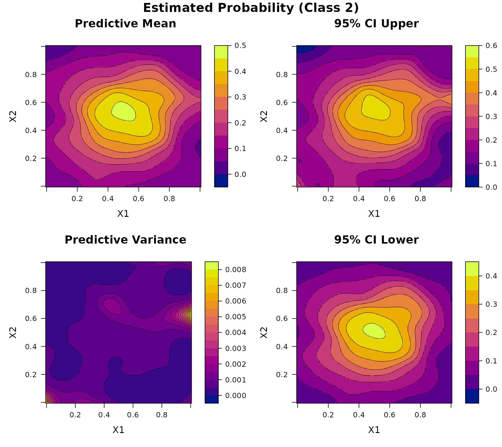
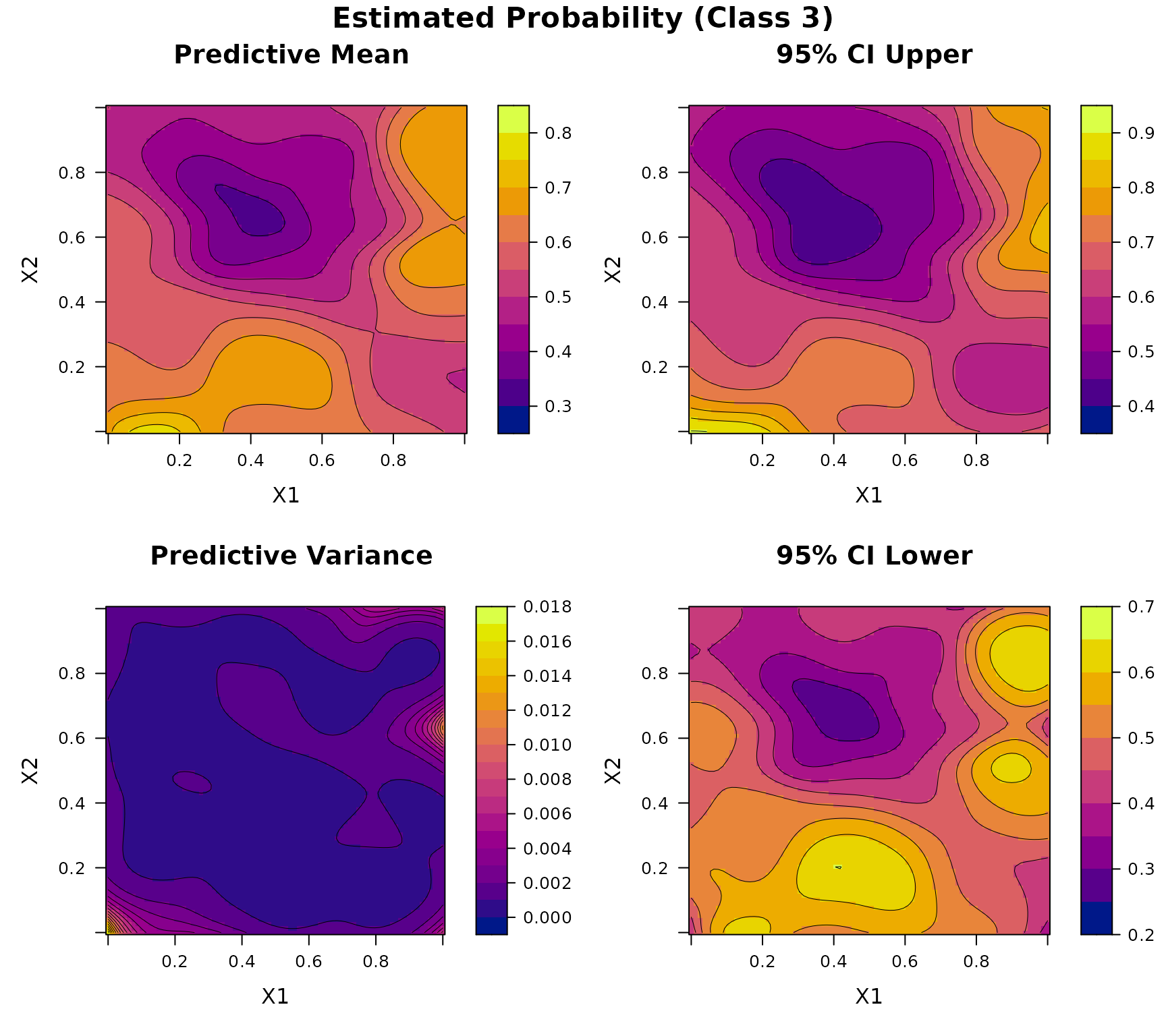
Consider a two-dimensional three-class classification problem. Let , and define the true class probability function as where is defined in Example 3, and We generate input points using Latin hypercube sampling over . At each location, the response is a multinomial vector with probability and a total count randomly sampled from .
set.seed(123)
# Define 2D latent function and probability transformation (3-class)
true_pi_fun_1 <- function(X) {
  if(is.null(nrow(X))) X <- matrix(X, nrow=1)
  m <- 8.6928
  s <- 2.4269
  x1 <- 4*X[,1]- 2
  x2 <- 4*X[,2]- 2
  a <- 1 + (x1 + x2 + 1)^2 *
    (19- 14*x1 + 3*x1^2- 14*x2 + 6*x1*x2 + 3*x2^2)
  b <- 30 + (2*x1- 3*x2)^2 *
    (18- 32*x1 + 12*x1^2 + 48*x2- 36*x1*x2 + 27*x2^2)
  f <- log(a*b)
  f <- (f- m)/s
  return(pnorm(f))  # Transform to probability
}
true_pi_fun <- function(X){
  p1 <- true_pi_fun_1(X)
  p2 <- sin(pi * X[,1]) * cos(pi * (X[,2] - 0.5))
  return(matrix(c(p1/2, p2/2, 1 - (p1+p2)/2), nrow = length(p1)))
}
n <- 100
Xbounds <- matrix(c(0, 0, 1, 1), nrow = 2)
X <- lhs(n = n, rect = Xbounds)
true_pi <- true_pi_fun(X)
m <- sample(150, n, replace = TRUE)
Y <- t(sapply(1:n, function(i) rmultinom(1, size = m[i], prob = true_pi[i, ])))

# Fit DKP model
DKP_model_2D <- fit.DKP(X, Y, Xbounds=Xbounds)

# Plot results
plot(DKP_model_2D)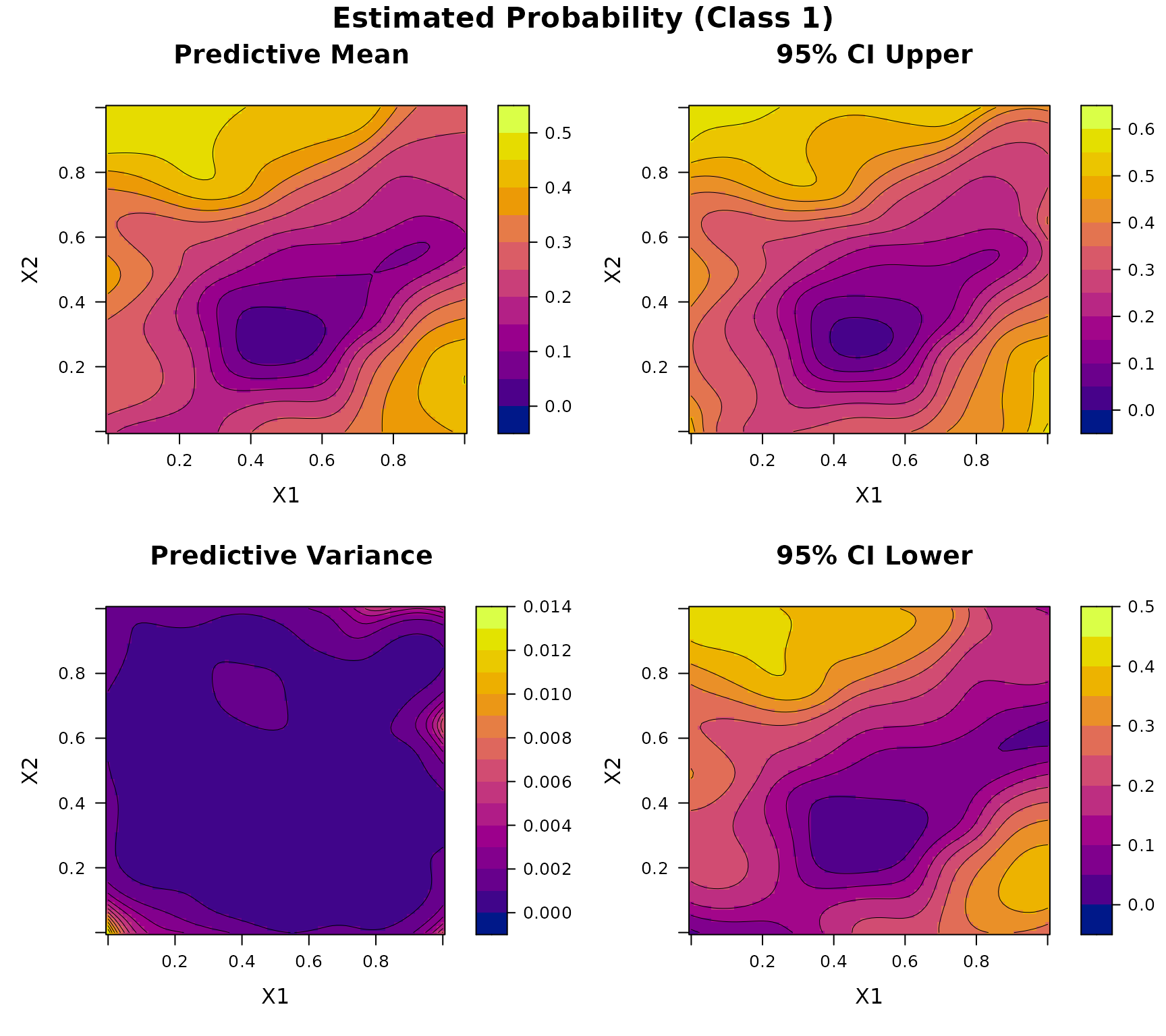
Example 7
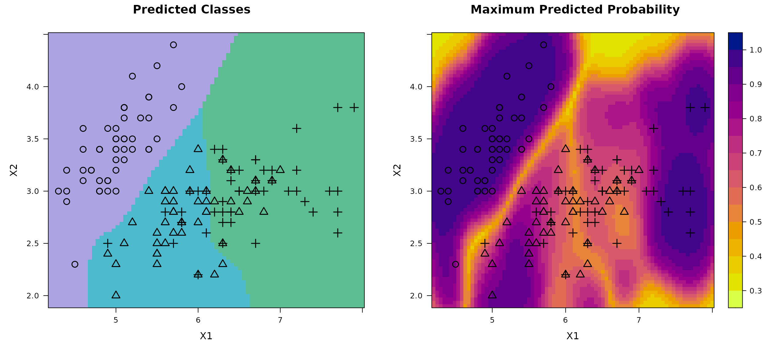
Consider another three-class classification task based on the well-known Iris dataset. This classic benchmark dataset contains measurements of three iris species (setosa, versicolor, and virginica) each described by four features: sepal length, sepal width, petal length, and petal width. Due to the overlap in feature space, particularly between versicolor and virginica, the class boundaries are not linearly separable, making this dataset a standard testbed for evaluating multi-class classification algorithms. For visualization purposes, we restrict our analysis to the first two features: sepal length and sepal width.
set.seed(123)
# Data
data(iris)
X <- as.matrix(iris[, 1:2])
Xbounds <- rbind(c(4.2, 8), c(1.9, 4.5))
labels <- iris$Species
Y <- model.matrix(~ labels - 1) # expand factors to a set of dummy variables

# Fit model
DKP_model_Class <- fit.DKP(
  X, Y, Xbounds = Xbounds, loss = "log_loss",
  prior = "fixed", r0 = 0.1, p0 = rep(1/3, 3))

# Plot results
plot(DKP_model_Class)