Plot Fitted BKP or DKP Models

Visualizes fitted BKP or DKP models depending on the input dimensionality. For 1-dimensional inputs, it displays predicted class probabilities with credible intervals and observed data. For 2-dimensional inputs, it generates contour plots of posterior summaries.

Usage

# S3 method for class 'BKP'
plot(x, only_mean = FALSE, ...)

# S3 method for class 'DKP'
plot(x, only_mean = FALSE, ...)

Arguments

x: An object of class "BKP" or "DKP", typically returned by fit.BKP or fit.DKP.
only_mean: Logical. If TRUE, only the predicted mean surface is plotted for 2D inputs (only applies to BKP models). Default is FALSE.
...: Additional arguments passed to internal plotting routines (currently unused).

Value

This function does not return a value. It is called for its side effects, producing plots that visualize the model predictions and uncertainty.

Details

The plotting behavior depends on the dimensionality of the input covariates:

1D inputs:
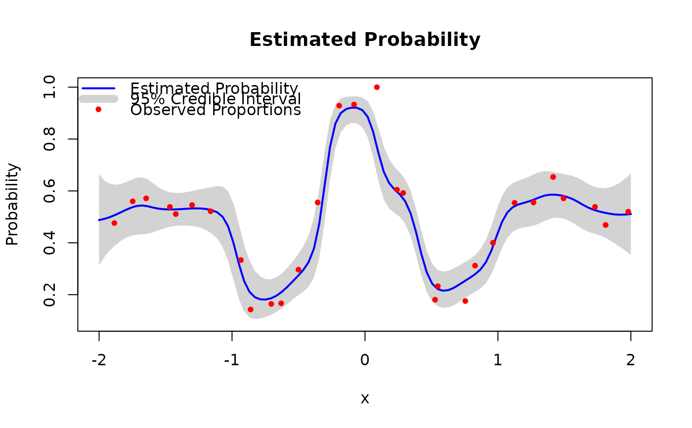
- For BKP, the function plots the posterior mean curve with a 95% credible band, along with the observed proportions (\(y/m\)).
- For DKP, the function plots one curve per class, each with a shaded credible interval and observed multinomial class frequencies.
2D inputs:
- For both models, the function produces a 2-by-2 panel of contour plots for each class (or the success class in BKP), showing:
  1. Predictive mean surface
  2. Predictive 97.5th percentile surface (upper bound of 95% credible interval)
  3. Predictive variance surface
  4. Predictive 2.5th percentile surface (lower bound of 95% credible interval)

For input dimensions greater than 2, the function will terminate with an error.

Examples

# ============================================================== #
# ========================= BKP Examples ======================= #
# ============================================================== #

#-------------------------- 1D Example ---------------------------
set.seed(123)

# Define true success probability function
true_pi_fun <- function(x) {
  (1 + exp(-x^2) * cos(10 * (1 - exp(-x)) / (1 + exp(-x)))) / 2
}

n <- 30
Xbounds <- matrix(c(-2,2), nrow=1)
X <- tgp::lhs(n = n, rect = Xbounds)
true_pi <- true_pi_fun(X)
m <- sample(100, n, replace = TRUE)
y <- rbinom(n, size = m, prob = true_pi)

# Fit BKP model
model1 <- fit.BKP(X, y, m, Xbounds=Xbounds)

# Plot results
plot(model1)



#-------------------------- 2D Example ---------------------------
set.seed(123)

# Define 2D latent function and probability transformation
true_pi_fun <- function(X) {
  if(is.null(nrow(X))) X <- matrix(X, nrow=1)
  m <- 8.6928
  s <- 2.4269
  x1 <- 4*X[,1]- 2
  x2 <- 4*X[,2]- 2
  a <- 1 + (x1 + x2 + 1)^2 *
    (19- 14*x1 + 3*x1^2- 14*x2 + 6*x1*x2 + 3*x2^2)
  b <- 30 + (2*x1- 3*x2)^2 *
    (18- 32*x1 + 12*x1^2 + 48*x2- 36*x1*x2 + 27*x2^2)
  f <- log(a*b)
  f <- (f- m)/s
  return(pnorm(f))  # Transform to probability
}

n <- 100
Xbounds <- matrix(c(0, 0, 1, 1), nrow = 2)
X <- tgp::lhs(n = n, rect = Xbounds)
true_pi <- true_pi_fun(X)
m <- sample(100, n, replace = TRUE)
y <- rbinom(n, size = m, prob = true_pi)

# Fit BKP model
model2 <- fit.BKP(X, y, m, Xbounds=Xbounds)

# Plot results
plot(model2)


# ============================================================== #
# ========================= DKP Examples ======================= #
# ============================================================== #

#-------------------------- 1D Example ---------------------------
set.seed(123)

# Define true class probability function (3-class)
true_pi_fun <- function(X) {
  p <- (1 + exp(-X^2) * cos(10 * (1 - exp(-X)) / (1 + exp(-X)))) / 2
  return(matrix(c(p/2, p/2, 1 - p), nrow = length(p)))
}

n <- 30
Xbounds <- matrix(c(-2, 2), nrow = 1)
X <- tgp::lhs(n = n, rect = Xbounds)
true_pi <- true_pi_fun(X)
m <- sample(100, n, replace = TRUE)

# Generate multinomial responses
Y <- t(sapply(1:n, function(i) rmultinom(1, size = m[i], prob = true_pi[i, ])))

# Fit DKP model
model1 <- fit.DKP(X, Y, Xbounds = Xbounds)

# Plot results
plot(model1)


#-------------------------- 2D Example ---------------------------
set.seed(123)

# Define latent function and transform to 3-class probabilities
true_pi_fun <- function(X) {
  if (is.null(nrow(X))) X <- matrix(X, nrow = 1)
  m <- 8.6928; s <- 2.4269
  x1 <- 4 * X[,1] - 2
  x2 <- 4 * X[,2] - 2
  a <- 1 + (x1 + x2 + 1)^2 *
    (19 - 14*x1 + 3*x1^2 - 14*x2 + 6*x1*x2 + 3*x2^2)
  b <- 30 + (2*x1 - 3*x2)^2 *
    (18 - 32*x1 + 12*x1^2 + 48*x2 - 36*x1*x2 + 27*x2^2)
  f <- (log(a * b) - m) / s
  p <- pnorm(f)
  return(matrix(c(p/2, p/2, 1 - p), nrow = length(p)))
}

n <- 100
Xbounds <- matrix(c(0, 0, 1, 1), nrow = 2)
X <- tgp::lhs(n = n, rect = Xbounds)
true_pi <- true_pi_fun(X)
m <- sample(100, n, replace = TRUE)

# Generate multinomial responses
Y <- t(sapply(1:n, function(i) rmultinom(1, size = m[i], prob = true_pi[i, ])))

# Fit DKP model
model2 <- fit.DKP(X, Y, Xbounds = Xbounds)

# Plot results
plot(model2)